Geo-coding
Overview
Geospatial analysis is commonly used in analyzing healthcare data to identify patterns that vary by geography. In this guide we describe a process for transforming healthcare data to enable geospatial analysis of publicly available social determinants of health data. Once you follow this guide it's very easy to perform geospatial analysis of any metric (e.g. cost, utilization, outcomes, risk, etc.).
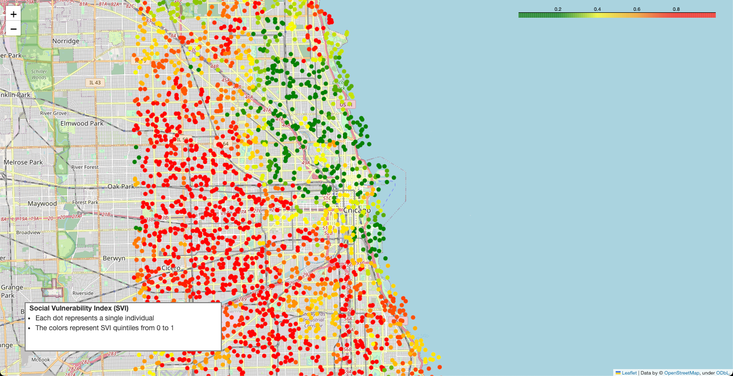
Below is an example of the types of geospatial visualizations that are easily produced by following this process. This guide doesn't show you how to create this visualization, but it does show you how to transform your data so that you can easily create this sort of visualization on your own.
Geo-coding
We start with patient data in a Snowflake database. For each patient we have an address, including street address, city, state, and zip code. The first step is geo-coding patient addresses i.e. converting them to latitude and longitude. We use AWS Location Services to perform geo-coding. Our process has the following workflow:
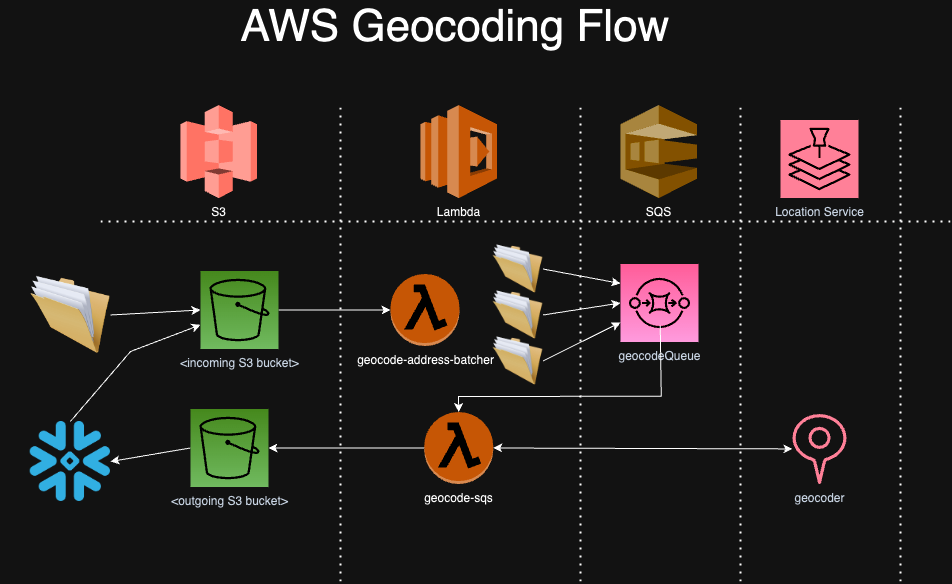
Most of the work in geo-coding involves deploying and managing cloud infrastructure and data pipelines shown in the diagram above. This infrastructure includes:
- Snowflake: Data warehouse that stores all patient data
- AWS S3: Cloud storage location where we send outbound data (from Snowflake that needs to be geo-coded) and inbound data (that has been geo-coded and needs to be loaded back into Snowflake)
- Lambda Address Batcher: Lambda function that breaks up address data into smaller batches so that AWS Location Services is more performant and sends those batches to the SQS Queue
- SQS: Queuing service that holds the batched address data for processing by Lambda and Location services
- Lambda Geo-coding: Lambda function that reads messages from the SQS Queue, runs them through AWS Location Services, then writes them back to S3
The geo-coding repository contains all the terraform code for creating the infrastructure and python code for the lambda functions upon which AWS Location Services will run. Instructions for deploying this code can be found in the README of this repository.
After setting up the infrastructure and lambda functions from the geo-coding repo, we need to create an AWS role that allows access to the S3 bucket you want to read from and write to. Full instructions for setting up the role are here. Then you then need to create a storage integration in Snowflake that uses that role. To create the storage integration:
create or replace storage integration <NAME>
  TYPE = EXTERNAL_STAGE
  STORAGE_PROVIDER = 'S3'
  ENABLED = TRUE
  STORAGE_AWS_ROLE_ARN = 'arn:aws:iam::<AWSACCOUNTNUM>:role/<ROLENAME>'
  STORAGE_ALLOWED_LOCATIONS = ('<S3BUCKET>')
Please make sure to replace:
- %lt;NAME%gt;
- %lt;AWSACCOUNTNUM%gt;
- %lt;ROLENAME%gt;
- %lt;S3BUCKET%gt;
Here is an example creation:
create or replace storage integration tuva
  TYPE = EXTERNAL_STAGE
  STORAGE_PROVIDER = 'S3'
  ENABLED = TRUE
  STORAGE_AWS_ROLE_ARN = 'arn:aws:iam::123456789123:role/aws-tuva-s3'
  STORAGE_ALLOWED_LOCATIONS = ('s3://s3-example-bucket/')
For the rest of this example we will assume that in the terraform code above (from the geo-coding repo) you set your pre-geocode prefix to /pre_geocode and your post-geocode prefix to /post_geocode.
If you are using the Tuva Data Model you can unload outbound patient data to be geo-coded from Snowflake to AWS S3 with the following SQL:
copy into s3://s3-example-bucket/pre_geocode/
from (
    select
        PATIENT_ID,
        ADDRESS,
        CITY,
        STATE,
        ZIP_CODE
    from tuva.core.patient
    where address is not null
    )
storage_integration = tuva
file_format = (type = csv COMPRESSION = NONE SKIP_HEADER = 0
field_optionally_enclosed_by = '"')
HEADER = TRUE
overwrite = TRUE
The S3 trigger created from the geo-coding repo automatically triggers the geo-coding process. As soon as patient addresses land in the S3 bucket the lambda address batcher is triggered and processing begins. Once the geo-coding process has finished (you can monitor this in the AWS Console -> SQS Queue) you can create a table for the raw geo-coded data and read it back in as follows:
CREATE or replace TABLE tuva.geocoded.raw_geocoded (data VARIANT);
COPY INTO tuva.geocoded.raw_geocoded
FROM s3://s3-example-bucket/post_geocode/
storage_integration = tuva
FILE_FORMAT = (TYPE = 'JSON');
We then convert the JSON data into a table with separate columns:
create or replace table tuva.geocoded.geocoded_patients as (
select data:Patient_id::varchar as Patient_id, data:Latitude as Latitude, data:Longitude as Longitude
from tuva.geocoded.raw_geocoded
);
Census Tracts and Block Groups
Now that our patient data is geo-coded, we can join it to other geographic datasets using geospatial queries. Here we show how to assign patients to census block groups and census tracts using geospatial joins based on their latitude and longitude. You can download the shape files in the reference data section.
For detailed descriptions of the differences between State, County, Tract and Block Group and Zip Code please see here.
In order to create the geospatial tables in Snowflake it requires a special user defined function (UDF).
CREATE OR REPLACE FUNCTION tuva.geocoded.PY_LOAD_GEOFILE(PATH_TO_FILE string, FILENAME string)
returns table (wkb binary, properties object)
language python
runtime_version = 3.8
packages = ('fiona', 'shapely', 'snowflake-snowpark-python')
handler = 'GeoFileReader'
AS $$
from shapely.geometry import shape
from snowflake.snowpark.files import SnowflakeFile
from fiona.io import ZipMemoryFile
class GeoFileReader:
    def process(self, PATH_TO_FILE: str, filename: str):
        with SnowflakeFile.open(PATH_TO_FILE, 'rb') as f:
            with ZipMemoryFile(f) as zip:
                with zip.open(filename) as collection:
                    for record in collection:
                        if (not (record['geometry'] is None)):
                            yield ((shape(record['geometry']).wkb, dict(record['properties'])))
$$;
Once you have created the UDF you can use it to load the data into the tables. Here's how you can create a stage in Snowflake to do that:
CREATE OR REPLACE STAGE tuva.geocoded.CENSUS_BG_STAGE;

grant all PRIVILEGES on stage tuva.geocoded.CENSUS_BG_STAGE to accountadmin;
Remember to update the role you need to grant the permissions to.
Once the stage is created you need to upload the shapefiles to the stage.
PUT file:///Users/user/Downloads/us-census-tracts.zip @CENSUS_BG_STAGE AUTO_COMPRESS=FALSE;
Remember to adjust the path in the PUT command to match your download location.
Create the table:
create or replace table tuva.reference.census_tracts as
SELECT
to_geography(wkb, True) as geography,
properties
FROM
	table(tuva.core.PY_LOAD_GEOFILE
			(build_scoped_file_url
				(@CENSUS_BG_STAGE, 'us-census-tracts.zip'),
				                   'us-census-tracts.shp')
)
;
Next, repeat the process for the census block groups (you can reuse the same stage).
PUT file:///Users/user/Downloads/us-census-block-groups.zip @CENSUS_BG_STAGE AUTO_COMPRESS=FALSE;

create or replace table tuva.reference.census_block_groups as
SELECT
to_geography(wkb, True) as geography,
properties
FROM
	table(tuva.core.PY_LOAD_GEOFILE
			(build_scoped_file_url
				(@CENSUS_BG_STAGE, 'us-census-block-groups.zip'),
				                   'us-census-block-groups.shp')
);
Next we use special geospatial functions to compute whether a specific latitude and longitude combination is within a given census tract or block group. Note that these functions work in Snowflake but may not be available in every data warehouse. The GEOGRAPHY column is a special column that contains a list of points that creates a polygon.
The function st_contains returns TRUE if a specific point exists inside the polygon. We use the st_point function to create that point using the longitude and latitude retrieved from the geo-coding process.
Census Tracts:
create or replace table tuva.geocoded.patient_tracts as (
select a.patient_id::varchar patient_id, b.PROPERTIES:GEOID::STRING FIPS
from tuva.geocoded.geocoded_patients a
join tuva.reference.census_tracts b
on st_contains(GEOGRAPHY, st_point(a.longitude, a.latitude))
);
Census Block Groups:
create or replace table tuva.geocoded.patient_block_groups as (
select a.patient_id::string patient_id, b.PROPERTIES:GEOID::STRING FIPS
from tuva.geocoded.geocoded_patients a
join tuva.reference.census_block_groups b
on st_contains(b.GEOGRAPHY, st_point(a.longitude, a.latitude))
);
This part of the query essential says "find the polygon that contains my point."
on st_contains(b.GEOGRAPHY, st_point(a.longitude, a.latitude))
Social Determinants
Now that we have transformed patient addresses into latitude and longitude and assigned each latitutde and longitude to a census tract and block group, we now need to join that data to the social determinants data we wish to analyze. Social determinants of health are commonly analyzed using geospatial techniques because these metrics tend to vary geographically.
Two publicly available social determinants datasets are the Social Vulnerability Index (SVI) and Area Deprivation Index (ADI) datasets, which contain a variety of metrics calculated at the census tract and census block group levels, respectively.
We make the SVI available for download as part of the Tuva Project. The ADI requires you to register and download it from the Neighborhood Atlas.
In order to load these files you need to first download them. You can download SVI from the reference dataset bucket, which you can find in the links above. Once you've done that you need to load them to a stage (you can re-use the same stage from the census files above) and then load them into your data warehouse.
PUT file:///Users/user/Downloads/SVI2020_US.csv @CENSUS_BG_STAGE AUTO_COMPRESS=FALSE;

create or replace table tuva.reference.svi (
    ST varchar, STATE varchar, ST_ABBR varchar, STCNTY varchar, COUNTY varchar, FIPS varchar
, LOCATION varchar, AREA_SQMI varchar, E_TOTPOP varchar, M_TOTPOP varchar, E_HU varchar
, M_HU varchar, E_HH varchar, M_HH varchar, E_POV150 varchar, M_POV150 varchar
, E_UNEMP varchar, M_UNEMP varchar, E_HBURD varchar, M_HBURD varchar, E_NOHSDP varchar
, M_NOHSDP varchar, E_UNINSUR varchar, M_UNINSUR varchar, E_AGE65 varchar, M_AGE65 varchar
, E_AGE17 varchar, M_AGE17 varchar, E_DISABL varchar, M_DISABL varchar, E_SNGPNT varchar
, M_SNGPNT varchar, E_LIMENG varchar, M_LIMENG varchar, E_MINRTY varchar, M_MINRTY varchar
, E_MUNIT varchar, M_MUNIT varchar, E_MOBILE varchar, M_MOBILE varchar, E_CROWD varchar
, M_CROWD varchar, E_NOVEH varchar, M_NOVEH varchar, E_GROUPQ varchar, M_GROUPQ varchar
, EP_POV150 varchar, MP_POV150 varchar, EP_UNEMP varchar, MP_UNEMP varchar, EP_HBURD varchar
, MP_HBURD varchar, EP_NOHSDP varchar, MP_NOHSDP varchar, EP_UNINSUR varchar, MP_UNINSUR varchar
, EP_AGE65 varchar, MP_AGE65 varchar, EP_AGE17 varchar, MP_AGE17 varchar, EP_DISABL varchar
, MP_DISABL varchar, EP_SNGPNT varchar, MP_SNGPNT varchar, EP_LIMENG varchar, MP_LIMENG varchar
, EP_MINRTY varchar, MP_MINRTY varchar, EP_MUNIT varchar, MP_MUNIT varchar, EP_MOBILE varchar
, MP_MOBILE varchar, EP_CROWD varchar, MP_CROWD varchar, EP_NOVEH varchar, MP_NOVEH varchar
, EP_GROUPQ varchar, MP_GROUPQ varchar, EPL_POV150 varchar, EPL_UNEMP varchar, EPL_HBURD varchar
, EPL_NOHSDP varchar, EPL_UNINSUR varchar, SPL_THEME1 varchar, RPL_THEME1 varchar, EPL_AGE65 varchar
, EPL_AGE17 varchar, EPL_DISABL varchar, EPL_SNGPNT varchar, EPL_LIMENG varchar, SPL_THEME2 varchar
, RPL_THEME2 varchar, EPL_MINRTY varchar, SPL_THEME3 varchar, RPL_THEME3 varchar, EPL_MUNIT varchar
, EPL_MOBILE varchar, EPL_CROWD varchar, EPL_NOVEH varchar, EPL_GROUPQ varchar, SPL_THEME4 varchar
, RPL_THEME4 varchar, SPL_THEMES varchar, RPL_THEMES varchar, F_POV150 varchar, F_UNEMP varchar
, F_HBURD varchar, F_NOHSDP varchar, F_UNINSUR varchar, F_THEME1 varchar, F_AGE65 varchar
, F_AGE17 varchar, F_DISABL varchar, F_SNGPNT varchar, F_LIMENG varchar, F_THEME2 varchar
, F_MINRTY varchar, F_THEME3 varchar, F_MUNIT varchar, F_MOBILE varchar, F_CROWD varchar
, F_NOVEH varchar, F_GROUPQ varchar, F_THEME4 varchar, F_TOTAL varchar, E_DAYPOP varchar
, E_NOINT varchar, M_NOINT varchar, E_AFAM varchar, M_AFAM varchar, E_HISP varchar
, M_HISP varchar, E_ASIAN varchar, M_ASIAN varchar, E_AIAN varchar, M_AIAN varchar
, E_NHPI varchar, M_NHPI varchar, E_TWOMORE varchar, M_TWOMORE varchar, E_OTHERRACE varchar
, M_OTHERRACE varchar, EP_NOINT varchar, MP_NOINT varchar, EP_AFAM varchar, MP_AFAM varchar
, EP_HISP varchar, MP_HISP varchar, EP_ASIAN varchar, MP_ASIAN varchar, EP_AIAN varchar
, MP_AIAN varchar, EP_NHPI varchar, MP_NHPI varchar, EP_TWOMORE varchar, MP_TWOMORE varchar
, EP_OTHERRACE varchar, MP_OTHERRACE varchar
);

copy into tuva.reference.svi from @CENSUS_BG_STAGE/SVI2020_US.csv
File_format = (type = CSV FIELD_OPTIONALLY_ENCLOSED_BY = '"'  SKIP_HEADER = 1);
PUT file:///Users/user/Downloads/US_2021_ADI_Census_Block_Group_v4_0_1.csv @CENSUS_BG_STAGE AUTO_COMPRESS=FALSE;

create table tuva.reference.adi (
  GISJOIN varchar
 ,FIPS varchar
 ,ADI_NATRANK varchar
 ,ADI_STATERNK varchar
);

copy into tuva.reference.adi from @CENSUS_BG_STAGE/US_2021_ADI_Census_Block_Group_v4_0_1.csv
File_format = (type = CSV FIELD_OPTIONALLY_ENCLOSED_BY = '"' SKIP_HEADER = 1);
Ready for Analysis
Now that you've 1) geo-coded patient addresses 2) assigned census tract and block groups and 3) loaded social determinants datasets, your data is ready for geospatial analysis. There are a wide variety of visualization tools, from R and python libraries to dashboards, that make this sort of analysis easy. We leave the choice of these tools to you as a next step. But the fruits of this labor are obvious in the SQL statements below. It's now very simple to join patients, geographic data, and social determinants data for analysis.
SVI:
create or replace table tuva.geocoded.patient_svi as (
select a.patient_id, b.*
from tuva.geocoded.patient_tracts a
join tuva.reference.svi b
on a.fips = b.fips
);
ADI:
create or replace table tuva.geocoded.patient_adi as (
select a.patient_id, b.*
from tuva.geocoded.patient_block_groups a
join tuva.reference.adi b
on a.fips = b.fips
);